Is Calibration Sufficient for Classification Models?

I recently read a blog post, which prompted a Twitter conversation about the importance of calibration in classification models. The conversation was intitiated based on this post from (538)[https://projects.fivethirtyeight.com/checking-our-work/] describing the calibration of their models using plots.

I am not going to argue whether or not 538’s specific use of calibration is a good way to evaluate their models. However, it is true that calibration is not sufficient for many applications in which the goal is discrimination (what I’m calling concordance to avoid the other negative meaning of the word). Jonathan Bartlett has an excellent blog post on why calibration may not be sufficient for classification models. I highly recommend that you read that post but the tdlr it’s possible to create a model that is well-calibrated but it omits a lot of information about that is predictive of the outcome. For example, a null model (one with out any covariates) may be well calibrated but wouldn’t be very useful. Essentially, the model would simply predict the base rate of the outcome, which would be less useful than a model that used some information in order to

When Concordance is Not Sufficient

Nevertheless, many statisticians posted replies that pushed back on the idea that calibration is overrated. For example, calibration can be very important in some applications particularly, when you’re trying to make a decision based on a cost / benefit analysis. Consequently, calibration can be especially useful in medicine (e.g. deciding whether a given intervention riskier than not performing it) or in the business (e.g. offering a discount to customers to prevent them from leaving).

One example of when concordance may not be sufficient is when their a uniform shift in the probability of the outcome. This phenonmen actually occured in my own work, when building a logistic regression model to predict the risk of high school dropout based on middle school grades and attendance. I built the model by training on a particular cohort and then testing the model on several subsequent. I arrived at an AUC of .87 both in the training data and the test data, indicating that the model performed well out of sample. However, while the training data was well calibrated, the model overestimated the dropout rate in the test data. How can this be?

Set Up

Here I define a logistic function to convert log odds to probabilities. I also created a calibration plot function. I think there are

library(pROC)

## Type 'citation("pROC")' for a citation.

## 
## Attaching package: 'pROC'

## The following objects are masked from 'package:stats':
## 
##     cov, smooth, var

logistic <- function(x) 1 / (1 + exp(-x)) # logistic function for converting log odds to probabilities


calibrate_plot <- function(y, y_hat,  bin_width) {
  
    bin_cuts <- seq.int(0,1, bin_width) # cutoff points for bins
    mid_pts <- ((bin_cuts + (bin_cuts  +bin_width)) / 2)[-length(bin_cuts)] #mid pt formula (drop last one )

    grp_mids <- cut(y_hat, bin_cuts) # group the predictions into bins for x-axis
    y_means <-  tapply(y, grp_mids, mean) # calculate the mean of each bin on the response variable for y -axi

    plot(mid_pts,  y_means, xlim = c(0,1), ylim = c(0,1)) #plot y_means over mid points
    abline(0, 1, lty = 'dashed', col = 'red') # add 45 degree line for reference
}


n <- 1e3 # Set sample size

Generate Data

I generated two predictors from a standardized normal distribution. I used these two predictor variables plus random noise to generate the log odds of my outcome.

\[ log odds (y) = B_{1} X_{1} + B_{2} x_{2} +\epsilon \]

# Generate Data
x1 <- rnorm(n) # predictor variable
x2 <- rnorm(n)  # predictor variable
logit_y <- 2*x1 + x2  +  rnorm(n) # log odds of outcome

Next I used my logistic function to convert

pr_y <- logistic(logit_y) #probability of outcome
y <- rbinom(n, 1, pr_y) # actual outcome
dta <- data.frame(y, x1, x2) # store as dta frame

Build and Evaulate model from Training Data Years

The data represented

I used logistirc regression to predict the probabilities of each

# Build and Evaulate Model
mod0 <- glm(y~ x1 + x2, dta, family = "binomial") # fit model
dta$y_hat <- predict(mod0, type = 'response') # predict probabilities given predictors

Evaluating Model in Training Years

I used the roc function from the pROC library to create a roc object. Then I plotted the

roc0 <- roc(dta, "y", "y_hat") # create roc object

## Setting levels: control = 0, case = 1

## Setting direction: controls < cases

plot(roc0)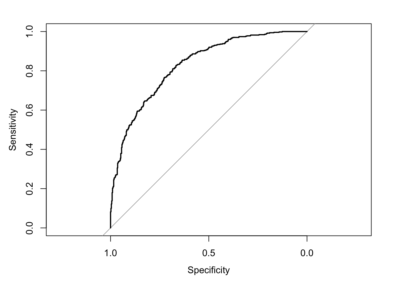

As you can see I arrive at a . As you probably already know, a predictive model with anAUC above .8 is generally considered to be pretty good.

auc(roc0) # calculate AUC

## Area under the curve: 0.8292

In the real world, I would probably want to test this model using training/test split to evaluate how the model

Testing Model

# Generate data for new time frame with slightly different timeframe
x1<- rnorm(n)
x2<- rnorm(n)
logit_y <- -1 + 1.8*x1+ 0.8*x2 + rnorm(n)
pr_y <- logistic(logit_y)
y <- rbinom(n, 1 , pr_y)
dta1 <- data.frame(y,  x1, x2)


# Make predictions basexsd on original model 
dta1$y_hat <- predict( mod0, newdata =dta1, type = 'response')

# Calculate AUC
roc1 <- roc(dta1, 'y', 'y_hat') 

## Setting levels: control = 0, case = 1

## Setting direction: controls < cases

auc(roc1)

## Area under the curve: 0.8467

Calibration

calibrate_plot(dta$y, dta$y_hat, 0.05)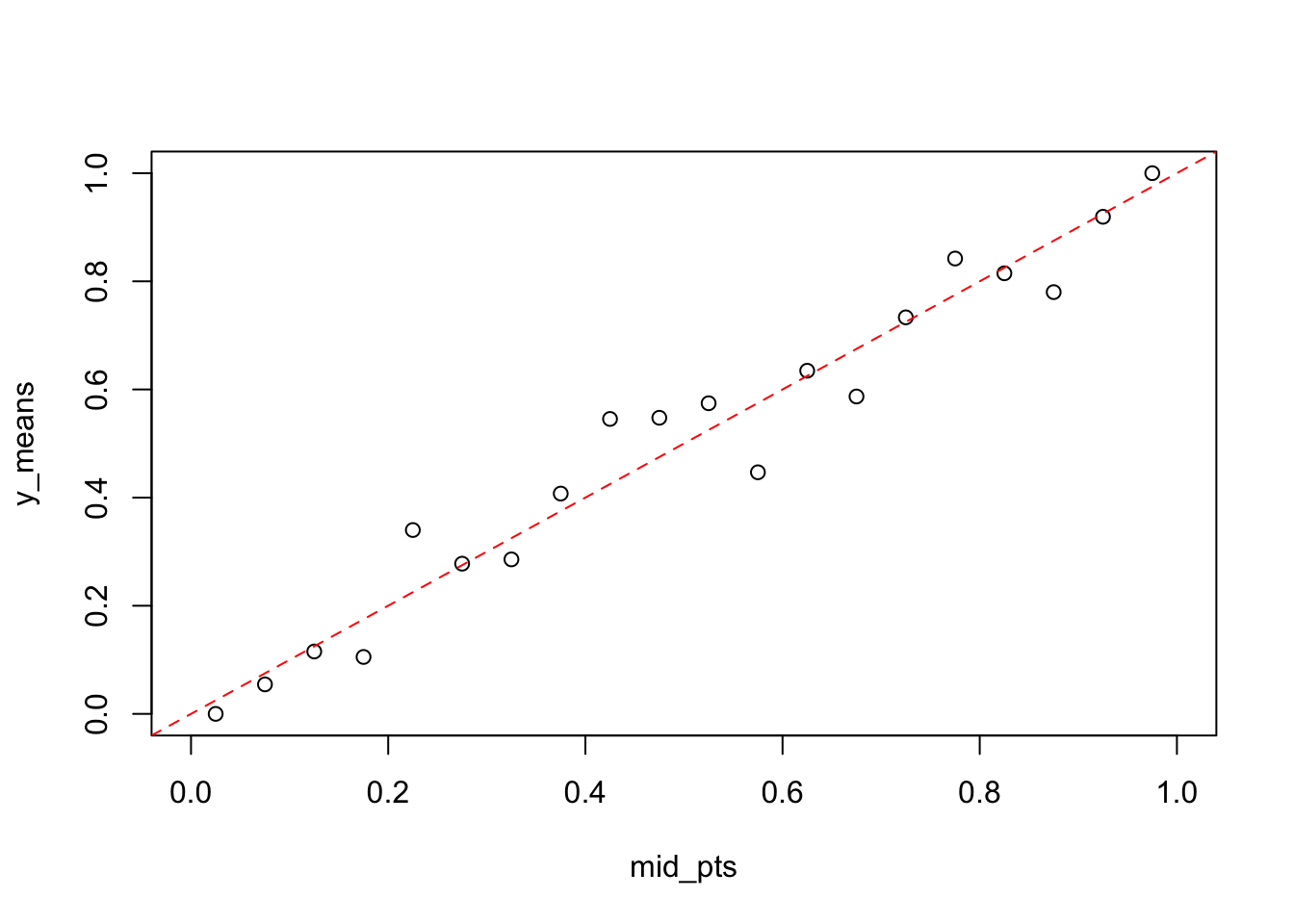

calibrate_plot(dta1$y, dta1$y_hat, 0.05)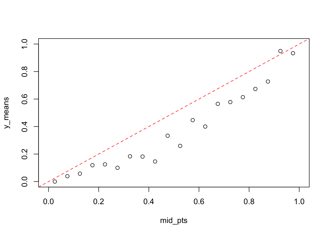

mean(dta1[dta1$y_hat > .9 , ]$y)

## [1] 0.9423077

mean(dta[dta$y_hat > .9 , ]$y)

## [1] 0.9509804